Image Tokens: Pixels Pay Tax Too
A live resolution→Token calculator; 32-pixel alignment tier jumps, the resolution curse, and three image-cost red lines
THE QUESTION THIS PAGE ANSWERS
ANSWER FIRSTWhat is the key idea behind “Image Tokens: Pixels Pay Tax Too”?
A live resolution→Token calculator; 32-pixel alignment tier jumps, the resolution curse, and three image-cost red lines
Read cost as a shape, not a single number. Break a request into input, output, retries, tools, and waiting time. The shape of usage usually tells you which design choice is expensive and where a smaller change can help.
Measure one real request before you optimize an imagined average.
A cheaper call that quietly creates more retries, latency, or review work.
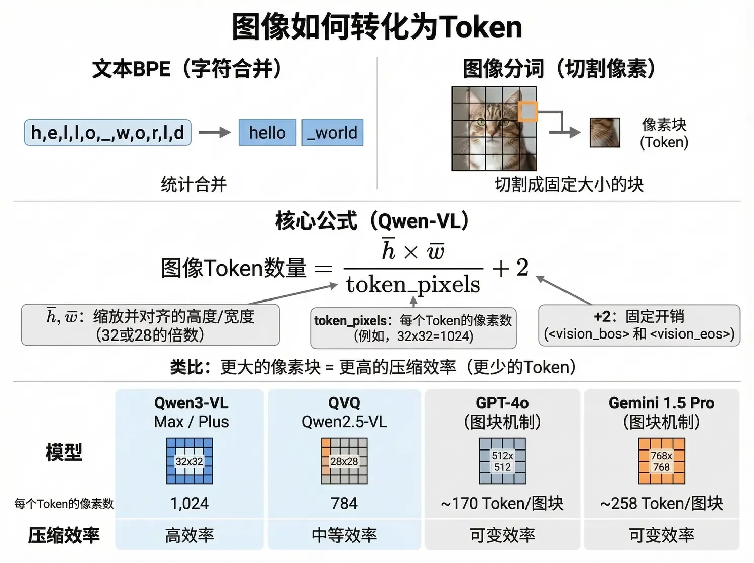
Vision models convert images into patches or tiles; each implementation maps visual regions to a model-specific number of Tokens. For one patch-based vision encoder, the teaching formula is:
| Variable | Meaning | Notes |
|---|---|---|
| h̄ / w̄ | Height & width after scaling | Often aligned to implementation-specific patch boundaries |
| token_pixels | Pixels per Token | This worksheet uses 32×32=1,024; other vision models use different patch or tile rules |
| +2 | Fixed overhead | Vision start/end markers <vision_bos> and <vision_eos> |
Other providers use tile mechanisms with their own image-detail modes and billing rules. The general principle is stable: text compression is shaped by vocabulary and merge rules; image compression is shaped by patch or tile size. Always read the target model's vision-tokenization and pricing documentation.
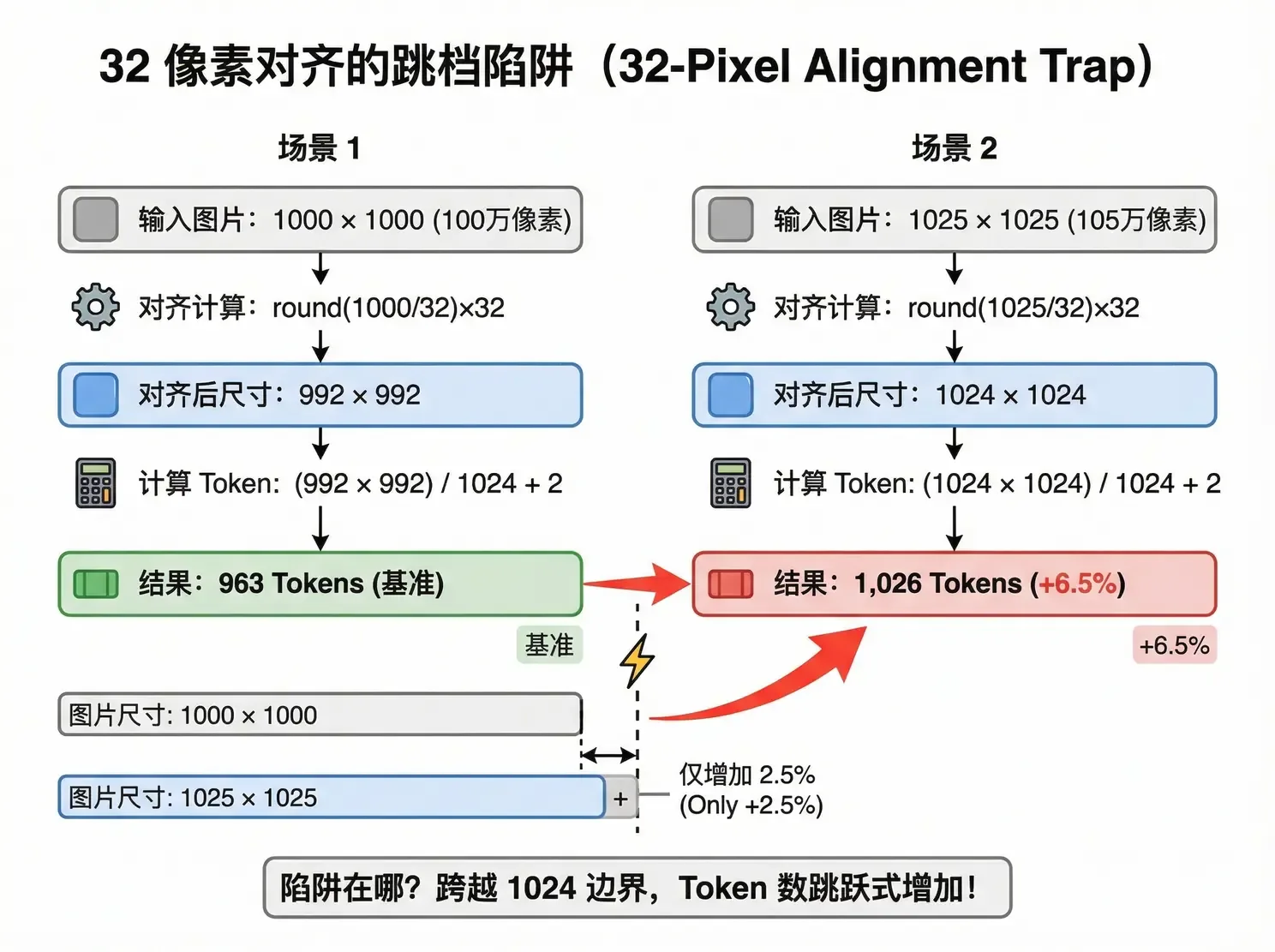
Pick a common resolution, or drag width and height yourself. Watch the “twin trap” of 1000×1000 vs 1025×1025. Billing assumption: this worksheet uses token_pixels = 1,024 and an illustrative input rate of $1/M within a 32k tier.
Is a 4K image better than 1080p? Not necessarily—and usually not worth it.
| Resolution | After scale (32-align) | Token count | Relative cost |
|---|---|---|---|
| 512 × 512 | 512 × 512 | 258 | 1x |
| 1080p (1920×1080) | 1920 × 1088 | 2,042 | 7.9x |
| 2K (2560×1440) | 2560 × 1440 | 3,602 | 14x |
| 4K (3840×2160) | 3840 × 2176 | 8,162 | 31.6x |
| 8K (7680×4320) | Hits scale cap | ~16,384 | 63.5x |
From 512 to 1080p, Tokens jump ~8× and recognition clearly improves; from 2K to 4K, Tokens roughly double again while accuracy gains may be invisible. You think you're paying for “sharper”—you're paying for “more pixel blocks”—and those extra blocks help the model less and less. Studies put VLM visual-Token redundancy as high as 85%.
| Task type | Token budget | Target resolution | Why |
|---|---|---|---|
| Coarse classification (cat vs dog) | < 300 | 512 × 512 | No detail needed |
| Scene understanding (what's happening) | < 1,000 | ~1000 × 1000 | Enough |
| OCR / chart analysis | < 4,000 | ~2000 × 2000 | Need to read text |
| High-precision detection (medical imaging) | < 16,384 | 4K+ | Enable the provider's high-resolution option as needed |
Three moves on the ground: front-end pre-compress (shrink to the target Token budget before upload; hold the resolution red line), task tiering (match the table—don't use 4K for classification), multi-image budget pool (when batch Tokens near 32k, truncate—same logic as last lesson's RAG budget cut).
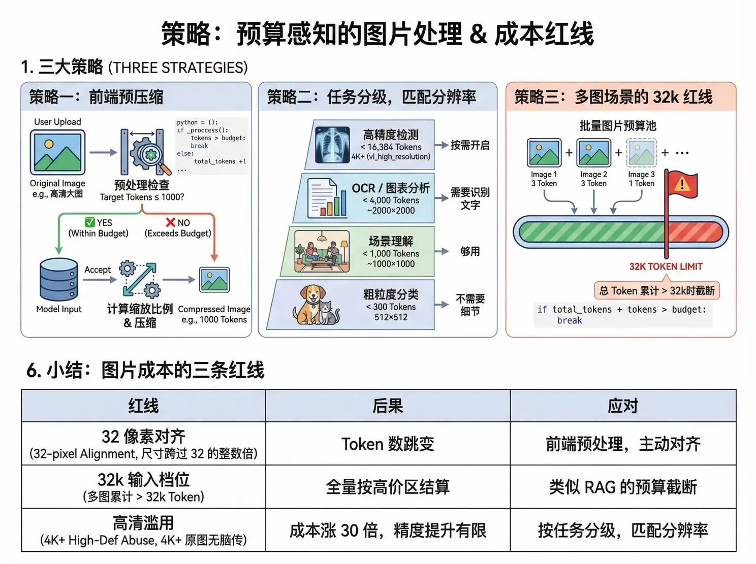
| Red line | Threshold | Consequence | Response |
|---|---|---|---|
| 32-pixel alignment | Size crosses a multiple of 32 | Token count jumps | Front-end preprocess; align proactively |
| 32k input tier | Multi-image total > 32k Tokens | Whole request bills in the expensive band | Budget truncation like RAG |
| HD abuse | Blindly sending 4K+ originals | Cost ×30, limited accuracy gain | Match resolution to task tier |
Images bill the resolution after scale-and-align, not the original you upload. Formula: (h̄×w̄)/token_pixels + 2.
High-res returns diminish: 4K costs ~4× 1080p and may not understand better. Match resolution to task tier.
Multi-image needs a budget pool: near 32k, truncate or compress—don't let the 5th image drag the whole bill into the expensive band.
Source: Adapted from the author's internal team share “AI Token Cost Engineering Strategies,” section “Image Token Billing.” The figures are an illustrative patch-based worksheet, not a universal billing rule; compare the target provider's official vision-tokenization and pricing docs, such as OpenAI image inputs, Google Gemini token guidance, and Alibaba Cloud Model Studio vision docs. Academic source for the “resolution curse”: CARES paper.
The complete interaction cost of “How images become Tokens”
“Vision models convert images into patches or tiles;” is a reminder that AI cost is not one price multiplied by one call. Input, output, retries, tools, waiting time, and human cleanup together decide what a task really costs.
Find what the bill repeats
The key variables behind “Other providers use tile mechanisms with their own image-detail modes and billing rules.” are usually repeated context, oversized output, retries after failure, and calls that do not produce useful progress. Removing wasted Tokens can reduce cost, latency, and concurrency pressure at the same time.
A cheaper call can make the whole workflow more expensive
Start with “Multi-image needs a budget pool: near 32k, truncate or compress—don't let the 5th image drag the whole bill into the expensive band” and keep a small table for input, output, retries, tools, and human review. Compare quality before and after optimizing instead of looking at one price in isolation.
From “How images become Tokens” to “Interactive Demo · How many Tokens is your image worth”
“How images become Tokens” grounds the problem in “Vision models convert images into patches or tiles; each implementation maps visual regions to a model-specific number of Tokens. For one patch-based vision encoder, the teaching formula is”. “Interactive Demo · How many Tokens is your image worth” then moves it toward “Pick a common resolution, or drag width and height yourself. Watch the “twin trap” of 1000×1000 vs 1025×1025. Billing assumption: this worksheet uses token_pixels = 1,024 and an illustrative input rate of $1/M…”. Together, they show that the lesson is not just a conclusion to remember, but a claim with conditions.
Carry the judgment into the next situation
When analyzing cost, map the complete interaction first, then find repeated input, wasted output, and retries. A cheap individual call does not make the whole task cheap.
- “How images become Tokens”: Vision models convert images into patches or tiles; each implementation maps visual regions to a model-specific number of Tokens. For one patch-based vision encoder, the teaching formula is
- “Interactive Demo · How many Tokens is your image worth”: Pick a common resolution, or drag width and height yourself. Watch the “twin trap” of 1000×1000 vs 1025×1025. Billing assumption: this worksheet uses token_pixels = 1,024 and an illustrative input rate of $1/M…
- “The closing point”: High-res returns diminish: 4K costs ~4× 1080p and may not understand better. Match resolution to task tier
The final “The closing point” brings the discussion to “High-res returns diminish: 4K costs ~4× 1080p and may not understand better. Match resolution to task tier”. The useful thing to carry forward is knowing which judgments must be revisited when input, scale, or risk changes.
I turned one judgment from this article into a small experiment I could run today. Knowing what to observe next is more useful than simply remembering the conclusion.
After reading this, I first looked for the conditions behind the idea instead of copying the method into a project. That order made the later trade-offs much clearer.
When this judgment reaches real work, which constraint should be added first? I am curious which step matters most between reading and the first practical attempt.
No discussion on this article yet.